Panda's Friends!
IPython
Numpy
Matplotlib

Pandas and Friends
Austin Godber
Mail: godber@uberhip.com
Twitter: @godber
Pandas is a Python data analysis tool built on top of NumPy that provides a suite of data structures and data manipulation functions to work on those data structures. It is particularly well suited for working with time series data.
Installing with pip or apt-get:
pip install pandas
# or
sudo apt-get install python-pandas
Mac - Homebrew or MacPorts to get the dependencies, then pip
Windows - Python(x,y)?, Commercial Pythons
IPython
Numpy
Matplotlib

Dependencies, required, recommended and optional
# Required
numpy, python-dateutil, pytx
# Recommended
numexpr, bottleneck
# Optional
cython, scipy, pytables, matplotlib, statsmodels, openpyxl
IPython is a fancy python console. Try running ipython or ipython --pylab on your command line. Some IPython tips
# Special commands, 'magic functions', begin with %
%quickref, %who, %run, %reset
# Shell Commands
ls, cd, pwd, mkdir
# Need Help?
help(), help(obj), obj?, function?
# Tab completion of variables, attributes and methods
There is a web interface to IPython, known as the IPython notebook, start it like this
ipython notebook
# or to get all of the pylab components
ipython notebook --pylab
Follow along by connecting to one of these servers.
NOTE: Only active on presentation day.
NumPy is the foundation for Pandas
Numerical data structures (mostly Arrays)
Operations on those.
Less structure than Pandas provides.
import numpy as np
# np.zeros, np.ones
data0 = np.zeros((2, 4))
#array([[ 0.,  0.,  0.,  0.],
#       [ 0.,  0.,  0.,  0.]])
data1 = np.arange(100)
#array([  0, 1, 2, .. 99])
data = np.arange(20).reshape(4, 5)
#array([[ 0,  1,  2,  3,  4],
#       [ 5,  6,  7,  8,  9],
#       [10, 11, 12, 13, 14],
#       [15, 16, 17, 18, 19]])
data.dtype    #dtype('int64')
result = data * 20.5
#array([[ 0. , 20.5, 41. , 61.5, 82. ], ...
#dtype('float64')
Tabular, Timeseries, Matrix Data - labeled or not
Sensible handling of missing data and data alignment
Data selection, slicing and reshaping features
Robust data import utilities.
Advanced time series capabilities
Series - 1D labeled array
DataFrame - 2D labeled array
Panel - 3D labeled array (More D)
In my code samples, assume I import the following
import pandas as pd
import numpy as np
See code/series_ex1.py for python source from which the next slides were derived.
one-dimensional labeled array
holds any data type
axis labels known asi index
dict-like
s1 = pd.Series([1, 2, 3, 4, 5])
# 0    1
# 1    2
# 2    3
# 3    4
# 4    5
# dtype: int64
print s1 * 5
# 0     5
# 1    10
# 2    15
# 3    20
# 4    25
# dtype: int64
print s1 * 5.0
# 0     5
# 1    10
# 2    15
# 3    20
# 4    25
# dtype: float64
s2 = pd.Series([1, 2, 3, 4, 5],
                index=['a', 'b', 'c', 'd', 'e'])
# a    1
# b    2
# c    3
# d    4
# e    5
# dtype: int64A quick aside ...
dates = pd.date_range('20130626', periods=5)
# <class 'pandas.tseries.index.DatetimeIndex'>
# [2013-06-26 00:00:00, ..., 2013-06-30 00:00:00]
# Length: 5, Freq: D, Timezone: None

dates[0]
# <Timestamp: 2013-06-26 00:00:00>s3 = pd.Series([1, 2, 3, 4, 5], index=dates) # 2013-06-26 1 # 2013-06-27 2 # 2013-06-28 3 # 2013-06-29 4 # 2013-06-30 5 # Freq: D, dtype: int64
Note that the integer index is retained along with the new date index.
s3[0]
# 1
s3[1:3]
# 2013-06-27    2
# 2013-06-28    3
# Freq: D, dtype: int64
s3[s3 < 3]
# 2013-06-26    1
# 2013-06-27    2
# Freq: D, dtype: int64
s3['20130626':'20130628']
# 2013-06-26    1
# 2013-06-27    2
# 2013-06-28    3
# Freq: D, dtype: int64
Things not covered but you should look into:
Other instantiation options: dict
Operator Handling of missing data NaN
Reforming Data and Indexes
Boolean Indexing
Other Series Attributes:
index - index.name
name - Series name
2-dimensional labeled data structure
Like a SQL Table, Spreadsheet or dict of Series objects.
Columns of potentially different types
Operations, slicing and other behavior just like Series
See code/dataframe_ex1.py for python source from which the next slides were derived.
data1 = pd.DataFrame(np.random.rand(4, 4))
#          0         1         2         3
# 0  0.748663  0.119829  0.382114  0.375031
# 1  0.549362  0.409125  0.336181  0.870665
# 2  0.102960  0.539968  0.356454  0.661136
# 3  0.233307  0.338176  0.577226  0.966152
dates = pd.date_range('20130626', periods=4)
data2 = pd.DataFrame(np.random.rand(4, 4),
                     index=dates, columns=list('ABCD'))
#                    A         B         C         D
# 2013-06-26  0.538854  0.061999  0.099601  0.010284
# 2013-06-27  0.800049  0.978754  0.035285  0.383580
# 2013-06-28  0.761694  0.764043  0.136828  0.066216
# 2013-06-29 0.129422 0.756846 0.931354 0.380510See? You never need Excel again!
data2['E'] = data2['B'] + 5 * data2['C']
#                    A         B         C         D         E
# 2013-06-26  0.014781  0.929893  0.402966  0.014548  2.944723
# 2013-06-27  0.968832  0.015926  0.976208  0.507152  4.896967
# 2013-06-28  0.381733  0.916911  0.828290  0.678275  5.058361
# 2013-06-29  0.447551  0.066915  0.308007  0.426910  1.606950
# Deleting a Column
del data2['E']

# Column Access as a dict
data2['B']
# or attribute
data2.B
# by row label
data2.loc['20130627']
# by integer location
data2.iloc[1]
data3 = pd.DataFrame(np.random.rand(400, 4))
data2.head()
#          0         1         2         3
# 0  0.245475  0.488223  0.624225  0.563708
# 1  0.237461  0.441690  0.162622  0.173519

data2.tail()
#          0         1         2         3
# 398  0.474941  0.847748  0.682227  0.871416
# 399  0.414240  0.819523  0.234805  0.333394
Like DataFrame but 3 or more dimensions.
Robust IO tools to read in data from a variety of sources
Matplotlib - The standard Python plotting tool
Trellis - An 'R' inspired Matplotlib based plotting tool
The csv file (code/phx-temps.csv) containing Phoenix weather data from GSOD:
1973-01-01 00:00:00,53.1,37.9
1973-01-02 00:00:00,57.9,37.0
...
2012-12-30 00:00:00,64.9,39.0
2012-12-31 00:00:00,55.9,41.0
# simple readcsv
phxtemps1 = pd.read_csv('phx-temps.csv')
# define index, parse dates, name columns
phxtemps2 = pd.read_csv('phx-temps.csv', index_col=0,
                        names=['highs', 'lows'],
parse_dates=True)import matplotlib.pyplot as plt
phxtemps2 = pd.read_csv('phx-temps.csv', index_col=0,
names=['highs', 'lows'],
parse_dates=True)
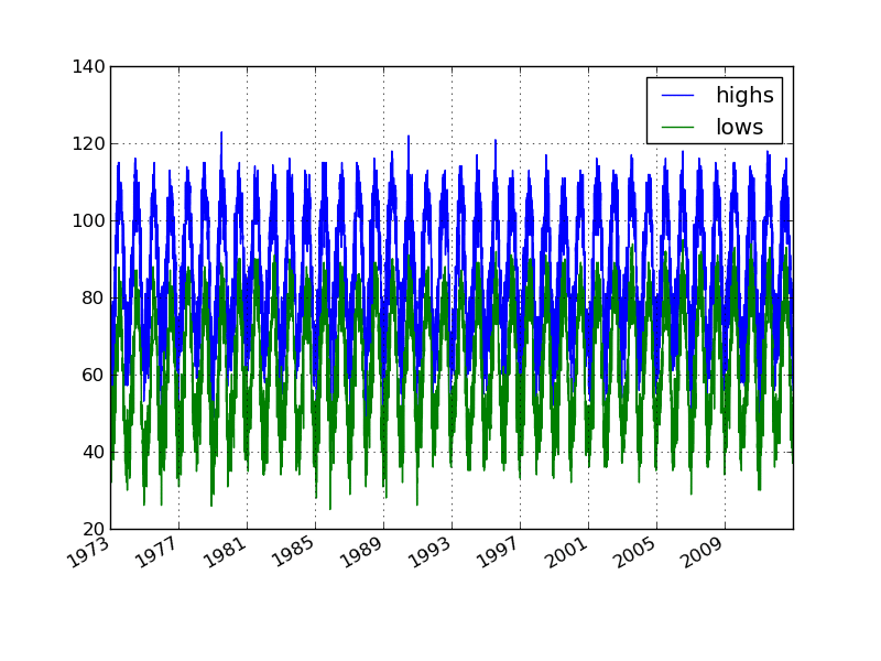
phxtemps2.plot() # pandas convenience method
plt.savefig('phxtemps2.png')

Boo, Pandas and Friends would cry if they saw such a plot.
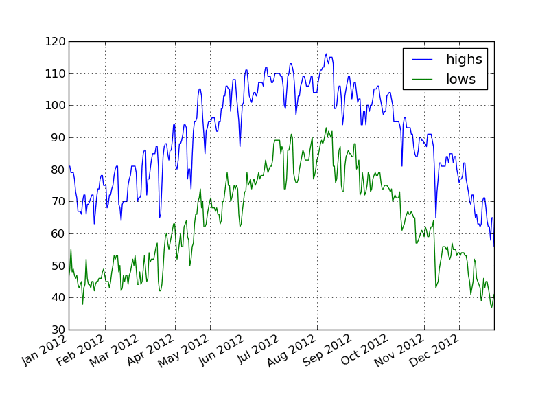
phxtemps2['20120101':'20121231'].plot()

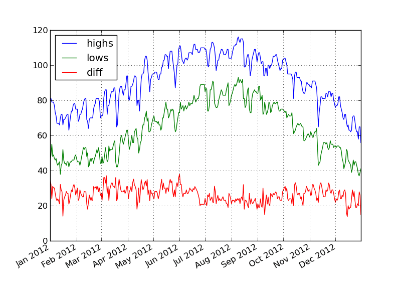
phxtemps2['diff'] = phxtemps2.highs - phxtemps2.lows
phxtemps2['20120101':'20121231'].plot()

AstroPy seems to have similar data structures.
I suspect there are others.
Presentation Source - https://github.com/desertpy/presentations